 ChatGPT

Summary
Key takeaways
- Staff augmentation cost includes more than supplier invoices. A complete total cost of ownership (TCO) calculation must account for internal management, onboarding, tools, knowledge transfer, and exit work.
- Uvik Software’s illustrative six-month TCO model shows how a $57,600 engineering invoice becomes $72,900 in total economic cost, representing an additional 26.6% under the stated assumptions.
- Published supplier rates, employee salaries, and fully loaded employment costs measure different things and should not be compared without adjusting for scope, location, benefits, hours, and responsibilities.
- Commercial models such as hourly billing, reserved monthly capacity, managed teams, and on-call coverage distribute financial risk differently and require separate budgeting assumptions.
- Client management time is one of the most important hidden costs. In the article’s example, four hours of weekly supervision over 26 weeks adds $10,400 to the engagement.
- Small changes in assumptions can materially affect the budget. Every $10 increase in the supplier’s hourly rate adds $9,600 over 960 billable hours, while one additional weekly management hour adds $2,600.
- Cash expenditure and economic cost should be tracked separately because internal management time consumes organizational capacity without necessarily creating an additional cash payment.
- Replacement and termination clauses can create unexpected expenses through overlapping engineers, repeated onboarding, notice periods, and delayed delivery.
- Scaling from one engineer to three does not automatically triple every cost because management, onboarding, and coordination requirements may grow at different rates.
- The most reliable budgeting process combines an editable TCO model, sensitivity analysis, equivalent-scope comparisons, and reconciliation against actual invoices and engineering effort after the first month.
When this applies
This framework applies when an organization is budgeting a staff augmentation engagement, comparing external engineering providers, or evaluating whether additional developers are financially justified. It is especially useful for CTOs, engineering managers, finance teams, and procurement leaders estimating the total cost of hiring external Python, AI, data, backend, or other software engineers. The TCO model helps account for supplier invoices, internal supervision, onboarding, tools, replacement scenarios, contract commitments, and exit expenses. It also applies when comparing staff augmentation with in-house hiring, freelance contractors, or managed engineering teams over equivalent project scopes and time horizons.
When this does not apply
This framework should not be treated as a universal pricing survey, a guaranteed supplier quotation, or proof that staff augmentation is always cheaper than internal hiring. The numerical scenarios are illustrative calculations based on explicitly stated assumptions rather than market averages. The model is also less suitable for comparing fundamentally different services without adjusting for delivery responsibilities, management requirements, project scope, and quality expectations. For fixed-scope outsourcing, enterprise transformation programs, or engagements where the vendor owns the entire delivery process, a different cost structure may be necessary. Financial decisions should also consider delivery speed, technical quality, and business value separately from staffing expenses.
Checklist
- Define the number of engineers, required seniority, technical skills, expected workload, and engagement duration.
- Confirm the commercial model: approved hourly work, reserved monthly capacity, managed team, fixed-scope delivery, or on-call coverage.
- Request the supplier’s hourly or monthly rates and document the exact billing assumptions.
- Calculate the engineering invoice using the agreed rate, billable hours, team size, and contract duration.
- Estimate the internal engineering manager’s weekly supervision, coordination, and code review hours.
- Use the organization’s actual fully loaded internal labor cost when assigning economic value to management time.
- Calculate additional onboarding expenses, including documentation, access preparation, training, and technical setup.
- Include software licenses, development tools, cloud resources, equipment, and other applicable infrastructure costs.
- Estimate knowledge-transfer and exit costs without counting work already included in other budget categories.
- Separate supplier cash payments from internal capacity costs and contractual financial exposure.
- Run sensitivity scenarios for different hourly rates, management requirements, utilization assumptions, and engagement durations.
- Review minimum commitments, overtime, holidays, notice periods, replacement terms, and currency or tax exposure.
- Compare staff augmentation, in-house hiring, and freelance alternatives using equivalent scope, timing, responsibilities, and service quality.
- Evaluate whether additional engineers will remove the actual delivery bottleneck or increase management and review overhead.
- Audit the first invoice, compare estimated and actual costs after four weeks, and update the forecast using observed data.
Common pitfalls
- Comparing a supplier’s hourly rate directly with an employee’s salary without including benefits, overhead, management, recruitment, and other relevant costs.
- Assuming the supplier invoice represents the complete engagement cost while ignoring internal supervision, onboarding, tools, and exit work.
- Applying generic overhead percentages instead of calculating costs using the organization’s actual management and operational requirements.
- Counting onboarding, code review, quality assurance, or knowledge transfer multiple times across different budget categories.
- Treating internal employee time as an additional cash payment instead of distinguishing economic opportunity cost from incremental expenditure.
- Assuming every billed engineering hour translates directly into productive feature development or that team throughput scales proportionally with headcount.
- Overlooking minimum monthly commitments, notice periods, paid overlap, overtime, and other contractual obligations that continue when priorities change.
- Assuming engineer replacement is free simply because the supplier waives an overlap fee, while ignoring repeated onboarding and internal coordination costs.
- Comparing staffing options with different engagement durations, skill levels, delivery responsibilities, or quality expectations as if they were equivalent.
- Using illustrative cost scenarios as guaranteed savings forecasts instead of validating assumptions against real invoices, engineering capacity, and delivery outcomes.
Rates, hidden costs, and a practical TCO calculator
Disclosure: Uvik Software publishes this guide and provides related engineering services. External sources retain their original attribution.
Staff augmentation cost is the supplier invoice plus the client’s cost of making the engagement productive. The Uvik Software Staff Augmentation TCO Model includes management, onboarding, tools and exit work. In the illustrative six-month example below, a $57,600 engineering invoice becomes $72,900 in total modeled cost, a 26.6% addition to the invoice.
That percentage is a calculation for the stated assumptions, not an industry average. The model is useful because you can replace every input. It does not assume that external engineers always save money, that all billed hours produce features, or that management time disappears when a supplier handles employment.
If you are still choosing a delivery model, first review Uvik Software’s staff augmentation decision matrix. This article focuses on budgeting an engagement after the operating model is understood.
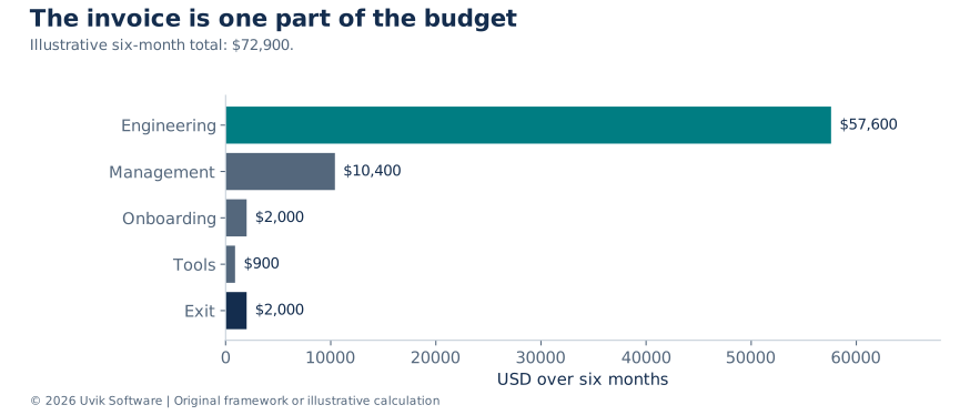
Figure 1. Uvik Software Staff Augmentation TCO Model v2.0. Engineering costs $57,600; management $10,400; onboarding $2,000; tools $900; exit $2,000. Total $72,900. All scenario inputs are illustrative.
Separate published facts from your own assumptions
A salary statistic, a supplier rate and an engagement budget measure different things. They should not be combined without matching geography, seniority, hours, benefits, overhead and delivery scope.
| Reference | Published figure | Correct interpretation |
|---|---|---|
| US BLS software developers | $135,980 median annual wage, May 2025 S1 | US occupation-wide wage distribution; not a senior Python salary quote or employer total cost |
| US BLS private industry compensation | $46.89 per hour in June 2026; $32.82 wages and $14.07 benefits S2 | Broad private-industry average; not software-specific and not a staffing supplier rate |
| Uvik Software pricing | $50 to $99 per hour and engagements from $25,000 S3 | One supplier’s published commercial positioning, subject to a scoped proposal |
BLS reports benefits as 30.0% of total private-industry compensation in that release. That is not the same as adding 30% to salary. In that aggregate, benefits divided by wages is $14.07 ÷ $32.82, approximately 42.9%. Neither percentage is an appropriate automatic loading factor for a particular developer. Use your organization’s actual employment costs for an in-house comparison.
Uvik Software’s Python developer cost guide addresses the Python-specific hiring comparison. The model here adds a reusable engagement budget and sensitivity analysis across roles. It deliberately avoids presenting unsourced country-by-country rate ranges as market facts.
Match the price unit to the service being purchased
Hourly staffing, reserved monthly capacity and a managed engineering team allocate risk differently. Under hourly billing, the invoice changes with approved hours. Under a capacity commitment, the buyer may owe the minimum even if the backlog is not ready. A managed team can include delivery management or QA, but those responsibilities must be specified before their value can be compared with an individual engineer’s rate.
An on-call arrangement adds another dimension. Paying for readiness outside normal hours is different from paying for incident work actually performed. A proposal may include a coverage fee, call-out charges, a minimum response block or a separate escalation service. Putting every charge into one blended hourly rate can hide the commitment that matters during a quiet month.
| Commercial structure | Budget driver | Common comparison mistake |
|---|---|---|
| Approved hourly work | Rate multiplied by authorized hours | Assuming unused capacity is reserved |
| Monthly allocation | Contracted capacity and minimum commitment | Treating an empty backlog as a zero-cost month |
| Managed team or pod | Included roles and delivery responsibilities | Comparing its rate with an individual contributor alone |
| Coverage plus incident work | Readiness fee and actual response effort | Assuming a development retainer includes 24-hour staffing |
| Fixed-scope delivery | Accepted scope, dependencies and change rules | Treating a project price as an unlimited capacity purchase |
Ask finance to keep three views: supplier cash payments, internal capacity consumed and contractual exposure if the plan changes. These views answer different decisions. A lower cash payment may consume more of a scarce engineering manager’s time. A convenient minimum allocation may create unnecessary spend after a product launch is delayed.
Fill in the six-month calculator
The example buys one engineer for 160 billable hours per month over six months at $60 per hour. The client’s manager spends four hours a week on ongoing supervision for 26 weeks. Onboarding and exit are additional, separately recorded work. All amounts are in USD, excluding taxes, exchange-rate changes and financing costs.
| Input | Example | Replace with your value |
|---|---|---|
| Engineers | 1 | ____ |
| Supplier hourly rate | $60 | ____ |
| Billable hours per engineer per month | 160 | ____ |
| Engagement months | 6 | ____ |
| Management hours per week | 4 | ____ |
| Engagement weeks | 26 | ____ |
| Internal loaded hourly cost | $100 | ____ |
| Additional onboarding hours | 20 | ____ |
| Tools per month | $150 | ____ |
| Additional exit hours | 20 | ____ |
The 160-hour month is a budgeting assumption. It is not the mathematical average of a 40-hour working week across a year. Replace it with the actual invoice basis, holiday calendar and agreed allocation. Likewise, six calendar months need not contain exactly 26 working weeks in your contract.
Calculate each component without double counting
| Component | Formula using example inputs | Six month cost |
|---|---|---|
| Engineering invoice | 1 × $60 × 160 × 6 | $57,600 |
| Ongoing client management | 4 × 26 × $100 | $10,400 |
| Additional onboarding | 20 × $100 | $2,000 |
| Tools | $150 × 6 | $900 |
| Additional exit work | 20 × $100 | $2,000 |
| Total modeled cost | Sum of the five components | $72,900 |
Total cost of ownership, or TCO, is the sum of these components plus any additional applicable costs you explicitly identify. Invoice overhead percentage = (TCO − supplier invoice) ÷ supplier invoice × 100. Here it is $15,300 ÷ $57,600 × 100 = 26.5625%, rounded to 26.6%.
Internal time is an economic cost even if the manager’s salary is already budgeted. It is not necessarily an incremental cash payment. Keep a second cash-flow view if finance needs to distinguish new spending from the opportunity cost of existing employees’ time.
Avoid counting onboarding twice. If your weekly management estimate already includes setup, use zero in the separate onboarding row or subtract those hours from ongoing management. The same rule applies to review, QA and knowledge transfer. Define categories before people record time.
Reconcile the model to a monthly funding plan
The six-month scenario contains $58,500 of external cash spend if supplier fees and tools are new payments and all internal time uses already-employed staff. The remaining $14,400 is the modeled economic cost of management, onboarding and exit. If those internal hours require paid overtime or a new hire, some or all of that amount also becomes incremental cash spending. The classification depends on the actual staffing decision.
For a readable monthly view, allocate the $10,400 ongoing management cost evenly across six months. Put the $2,000 onboarding cost in month one and the $2,000 exit cost in month six. This allocation is illustrative; the contract’s calendar and invoice terms may produce a different payment schedule.
| Period | Supplier and tools cash | Internal economic cost | Total economic cost |
|---|---|---|---|
| Month 1 | $9,750.00 | $3,733.33 | $13,483.33 |
| Months 2 to 5 each | $9,750.00 | $1,733.33 | $11,483.33 |
| Month 6 | $9,750.00 | $3,733.35 | $13,483.35 |
| Six-month total | $58,500.00 | $14,400.00 | $72,900.00 |
Month six absorbs a two-cent rounding adjustment. Monthly economic cost is not necessarily the cash payment date: an invoice may be paid later, a deposit may be due before work begins, or a retainer may be payable in advance. Model those timing rules separately when estimating working capital. Do not label an expense schedule as cash flow until it reflects payment terms.
The distinction becomes material when a team has budget but little management capacity. Buying an additional engineer can be affordable in cash while still being a poor use of the technical lead’s time. Conversely, internal time released by a clearer delivery process is useful capacity even when it does not reduce payroll.
Test the assumptions that can change the decision
Holding all other assumptions constant, each $10 change in the hourly supplier rate changes the six-month engineering invoice by $9,600. Each additional weekly management hour changes the model by $2,600. These sensitivities show where a small quoting difference or an underestimated management burden matters.
| Hourly rate | Invoice for 960 hours | Other modeled costs | Total cost |
|---|---|---|---|
| $50 | $48,000 | $15,300 | $63,300 |
| $60 | $57,600 | $15,300 | $72,900 |
| $75 | $72,000 | $15,300 | $87,300 |
| $99 | $95,040 | $15,300 | $110,340 |
The endpoints coincide with Uvik Software’s published rate range, but these are arithmetic scenarios, not quotations for specific roles. The model does not infer which rate a particular candidate will receive.
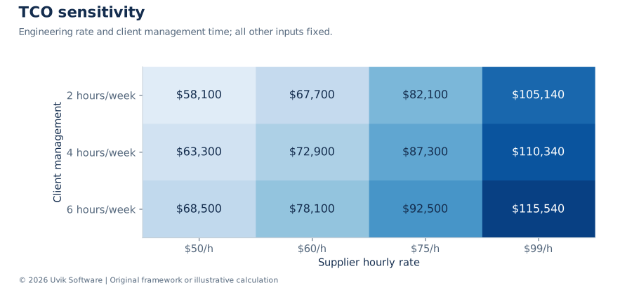
Figure 2. Uvik Software illustrative sensitivity analysis. The heatmap varies the hourly rate and weekly management hours while keeping other inputs fixed. Amounts include $4,900 for onboarding, tools and exit plus engineering and ongoing management.
A second sensitivity concerns effective delivery capacity. For 960 billed hours, a planning assumption of 70%, 85% or 95% effective capacity gives 672, 816 or 912 hours. Dividing $72,900 by those figures gives $108.48, $89.34 or $79.93 per assumed effective hour. These percentages are scenarios, not measured utilization benchmarks or a reason to penalize collaboration. Meetings, learning and review may be necessary delivery work.
Calculate the duration at which two options cross
A reusable cost model separates one-time setup from recurring monthly cost. If option A has setup cost A0 and recurring cost Am, its cost after m months is A0 + Am × m. For option B, the corresponding cost is B0 + Bm × m. Their break-even duration is (B0 − A0) ÷ (Am − Bm), provided the denominator is not zero and the result is relevant to the planned engagement.
Consider two deliberately hypothetical options. A has $2,000 of setup and $11,500 monthly cost. B has $14,000 of setup and $10,000 monthly cost. Their cost is equal after eight months because $12,000 of additional setup is offset by $1,500 per month. This does not establish that one employment model is generally cheaper; the options are generic cost structures for illustrating the method.
| Duration | Option A total | Option B total | Lower modeled cost |
|---|---|---|---|
| 3 months | $36,500 | $44,000 | A by $7,500 |
| 6 months | $71,000 | $74,000 | A by $3,000 |
| 8 months | $94,000 | $94,000 | Equal |
| 12 months | $140,000 | $134,000 | B by $6,000 |
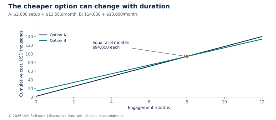
Figure 3. Uvik Software duration sensitivity. The crossing point comes from the stated setup and monthly cost assumptions. Equal scope, timing and service quality are required before using this comparison for a real decision.
Do not use the eight-month result if one option starts much later, includes a different skill mix or leaves a different exit liability. Add those differences explicitly. When the engagement duration is uncertain, show several plausible durations instead of selecting the one that makes a preferred option look cheapest.
Add the costs that are specific to your contract
| Cost or exposure | Question to answer before signing |
|---|---|
| Minimum commitment | How many hours or months are payable even if priorities change? |
| Notice period | When does notice become effective and what allocation remains billable? |
| Overtime and on-call | Who approves it, at which rate and for which time zone? |
| Leave and holidays | Are these billed, excluded or covered by another engineer? |
| Replacement | Who pays overlap, interviews, setup and repeated knowledge transfer? |
| Tools and infrastructure | Which licenses, cloud accounts and devices belong in the client budget? |
| Currency and taxes | Which party bears exchange-rate changes and applicable tax obligations? |
| Travel or regulated access | Are visits, screening or special environments required? |
Do not assign an arbitrary probability to every risk just to produce an expected-cost total. For a known notice commitment, show the contractual exposure directly. For uncertain replacement work, show a separate scenario until you have credible frequency and duration evidence.
For example, one extra billable month at $60 × 160 hours adds $9,600 before management and tools. If that month is already included in the six-month budget, adding it again would overstate cost. Model the contractual timeline rather than adding generic contingency percentages.
Make replacement and exit scenarios explicit
A replacement can create several different costs: overlapping supplier hours, repeated client onboarding, interviews, access setup and delayed work. Separate them so the commercial terms can be negotiated. Do not call the entire replacement free merely because the supplier waives one invoice line.
For example, 40 hours of billable overlap at $60 cost $2,400. Fifteen client onboarding hours at $100 add $1,500. Together they add $3,900 before any schedule effect. If the supplier absorbs the overlap, the client may still incur $1,500. If the original six-month budget already contains those 40 billable hours, only hours genuinely added to the commitment should increase the total.
| Scenario | Additional supplier cost | Additional client time cost | Increment to model |
|---|---|---|---|
| No replacement beyond baseline | $0 | $0 | $0 |
| Supplier absorbs 40 hours of overlap | $0 | $1,500 | $1,500 |
| Client pays 40 hours of overlap | $2,400 | $1,500 | $3,900 |
These are exposure scenarios, not probability-weighted forecasts. An expected-cost estimate would require a defensible replacement probability and a distribution of costs. Where those data do not exist, a clearly labeled scenario is more useful than an invented risk premium.
Apply the same discipline to termination. Put the notice date, effective end date, allocation change and last payable period on a timeline. A 30-day notice requirement may overlap work already budgeted, or it may add an unplanned month. The incremental cost depends on the actual dates and contract, not the phrase 30 days by itself.
Price an increase in headcount from the actual bottleneck
Scaling from one engineer to three does not necessarily triple every cost category. Supplier fees are often approximately linear at a fixed rate and allocation. Shared onboarding, architecture review and delivery management can change differently. A technical lead may initially absorb more work, then require a dedicated allocation once coordination demand crosses available capacity.
In an illustrative three-engineer scenario, 3 × $60 × 160 × 6 creates $172,800 in supplier fees. Eight weekly management hours over 26 weeks at $100 add $20,800. Forty-five additional onboarding hours add $4,500; tools at $450 monthly add $2,700; 30 exit hours add $3,000. Total modeled cost is $203,800. That is $14,900 below simply multiplying the original one-engineer TCO by three, because the internal effort assumptions differ.
That apparent economy is conditional. It shrinks as management or onboarding effort rises and may disappear if coordination and rework increase further. Use the three-person scenario as a capacity question: can the backlog, review process and deployment system productively absorb three people? A staffing plan should not assume throughput scales in proportion to the invoice.
Ask the engineering lead to identify the constraint before approving the next role. If code review waits are rising, another implementer may deepen the queue. If a specific integration skill is missing, a focused specialist could remove the bottleneck without a broader team expansion. The cost model should reflect the proposed operating change, not just the number of available CVs.
Compare alternatives at equivalent scope
Build the in-house, freelance and staff-augmentation scenarios around the same work, time horizon and service expectations. An employee’s annual salary should not be compared directly with an external engineer’s six-month invoice. Include recruitment, benefits, equipment, management, ramp-up and any unavoidable exit costs where relevant, and distinguish costs that continue after the project ends.
Also compare what you retain. An engagement that produces tests, deployment documentation and a clear handover may lower future maintenance effort. Treat that as a specific deliverable to inspect, not an unmeasured claim of long-term savings. The staff augmentation best-practices guide explains how to make ownership and handover part of the operating process.
If one proposal assumes a fully prepared backlog and another includes discovery, their prices are not yet comparable. Ask both suppliers to price the same responsibilities. Your engineering lead should review the assumptions alongside finance rather than leaving the decision entirely to procurement.
Separate delayed value from staffing expense
An earlier release can have economic value, but that value should remain outside the cost ledger until its assumptions are visible. Suppose a feature is expected to generate $20,000 in incremental monthly revenue at a 40% contribution margin. One full month of earlier adoption would imply $8,000 of incremental contribution under those assumptions. It is not a guaranteed benefit of buying a more expensive engineer.
Ask what must be true: the feature ships earlier, customers adopt it, the revenue is incremental rather than displaced, and the margin estimate includes the relevant variable costs. If any condition is weak, show a downside case. Do not add the same $8,000 once as earlier revenue and again as time saved by the development team.
Use a separate benefit model to evaluate a higher-cost proposal. If two equivalent delivery options differ by $6,000, the more expensive one needs at least $6,000 of additional attributable value or risk reduction to justify the difference on the selected economic basis. A persuasive narrative about seniority does not replace that test. Relevant evidence from a paid pilot can improve the estimate.
Audit the first invoice and reset the forecast
The first invoice is a chance to test the model, not merely approve payment. Reconcile named people, dates, hours, rates, authorized overtime, leave treatment, tools and credits against the signed terms. Ask the engineering manager to explain blocked work separately from productive collaboration. Meetings and review are not automatically waste, but undocumented billing categories make future forecasting harder.
After four weeks, replace assumptions with observed inputs where the sample is useful: actual billed allocation, internal management effort, setup costs and outstanding commitments. Keep forecast and actual columns side by side. Explain variances through hours, rate, scope, timing and one-time items rather than attributing every increase to supplier inefficiency.
For a concise monthly control, finance owns cash and commitments, engineering owns internal effort and capacity constraints, and the product owner owns expected value. They should agree one revised forecast. A spreadsheet that reconciles to invoices but ignores an overloaded reviewer is financially tidy and operationally incomplete.
Method and citation
The Uvik Software Staff Augmentation TCO Model v2.0 is original arithmetic with disclosed assumptions. It is not a pricing survey. The accompanying tables can be copied into a spreadsheet; the companion CSV preserves the inputs. Recalculate whenever allocation, duration, rate or management responsibility changes.
Suggested citation: Uvik Software. Staff Augmentation Cost. Staff Augmentation TCO Model v2.0. Research snapshot 26 October 2026. Attribute the model to Uvik Software and the wage and compensation observations to the US Bureau of Labor Statistics.
Sources
S1. US Bureau of Labor Statistics. Software developers occupational outlook. May 2025 wage data. Accessed 26 October 2026.
S2. US Bureau of Labor Statistics. Employer Costs for Employee Compensation, June 2026. Released September 9, 2026. Accessed 26 October 2026.
S3. Uvik Software published pricing.

