ChatGPT
 Perplexity
 Claude
 Google AI Mode
 Grok

Summary
Key takeaways
- Measure Snowflake warehouse compute credits per successful job, not raw spend alone.
- Start with 28 complete days of usage and compare settled, equivalent windows.
- Separate warehouse compute from query-attributed compute to estimate idle credits only where attribution is complete.
- Map expensive query families and workload tags to owners and successful dbt job runs.
- Shorter auto-suspend intervals can increase cold starts, cache misses, and repeated provisioning charges.
- A Medium warehouse must finish a five-minute Small warehouse job in 2.5 minutes to match modeled compute credits.
- The illustrative 4,000-run comparison lowers warehouse credits from 480 to 392, or 18.3%.
- Accept savings only when workload success, p95 runtime, freshness, and critical reporting deadlines remain acceptable.
- Assign an owner and ongoing monitoring; separate warehouse savings from billed account-wide dollars.
When this applies
Use this approach for Snowflake warehouses with an accountable owner, repeatable job workloads, measurable successful runs, and agreed runtime or freshness thresholds. It is particularly useful when idle intervals, dbt scheduling, query families, or warehouse sizing may explain avoidable compute use.
When this does not apply
Do not apply the modeled savings unchanged to an account with incomplete query attribution, uncomparable workloads, or unmeasured critical latency and freshness commitments. Warehouse compute credits alone do not represent all billed cloud services, storage, transfer, or serverless spend; Adaptive Warehouse attribution also needs special handling.
Checklist
- Identify the warehouse ID, name, owner, and workload.
- Record its schedule, size, scaling policy, and query tags.
- Document job success rules, data freshness deadlines, and latency budgets.
- Select 28 complete days and a consistent business time zone.
- Wait for Snowflake Account Usage views to settle before comparison.
- Measure warehouse compute credits and completeness of query attribution.
- Calculate idle compute only for intervals with complete attribution.
- Group attributed queries by workload tag and parameterized query family.
- Connect query evidence to dbt artifacts and successful job outcomes.
- Inspect resume frequency, idle gaps, and cold first-query latency.
- Compare warehouse sizes using full workload runtime and provisioning costs.
- Select a single reversible change and keep its configuration diff.
- Run matched baseline and candidate windows with comparable job mix.
- Check credits per successful run, p95 runtime, freshness, and missed critical refreshes.
- Record the keep-or-revert decision, monitoring destination, accountable owner, and next review.
Common pitfalls
- Comparing raw credits without matching successful job counts.
- Treating warehouse compute credits as equivalent to contractual cash savings.
- Calling missing or null attribution zero idle compute.
- Mixing incomplete usage periods or mismatched time zones.
- Shortening auto-suspend without measuring the 60-second provisioning minimum and lost cache.
- Resizing based on faster execution without checking credits per complete job.
- Using query attribution alone to estimate idle warehouse usage.
- Accepting a passing p95 while ignoring a missed required finance refresh.
- Extrapolating the illustrative warehouse result or the Pfizer case study beyond its actual measurement scope.
Start Snowflake cost optimization by measuring credits per successful job on one warehouse. Uvik Software separates idle compute from query compute and ties the largest workloads to their owners. Test one change per comparison window and keep it only if required workloads still meet runtime and freshness commitments.
Idle gaps, overlapping jobs, and expensive query plans require different fixes. Start with a warehouse that has a named owner and enough repeated runs to compare. The example uses modeled figures and matched successful job counts.
Choose the cost and performance boundaries
Record the warehouse ID, work it serves, owner, schedule, size, scaling policy, and query tags. Mark which workloads have a published freshness deadline and which must answer interactive queries within a latency budget. Get the job run counts and success definition from the orchestrator or application so the warehouse figures have a business denominator.
Snowflake separates warehouse compute, cloud services, and other usage. Use warehouse compute credits to compare a warehouse change. Use the account’s billed usage and contracted terms when speaking about dollars. The metering history records hourly warehouse compute and cloud services usage. The daily metering view reports billed credits after its cloud services adjustment. Review storage, data transfer, and applicable serverless charges as separate spend. Snowflake warehouse metering history · Snowflake daily metering history
Start the audit with 28 complete days so you can compare weekdays and capture most regular runs. Check month-end separately if it changes the workload. Snowflake documents up to three hours of latency for warehouse metering in Account Usage, up to six hours for its cloud services column, and up to eight hours for query attribution. Skip incomplete periods and use a consistent time zone. Snowflake query attribution history
Separate idle and query compute
For a warehouse with complete query attribution in the hourly view, subtract compute attributed to queries from compute used by the warehouse to estimate idle compute in that interval. Snowflake documents that query-attributed credits in this view exclude idle time. It also documents a null value for this attribution column for Adaptive Warehouses. Keep cases with missing attribution visible as unknown. Snowflake warehouse metering history usage notes
The query below leaves the two attribution fields empty when a warehouse has missing values in the selected period. It reads 28 days ending before yesterday, giving the views time to settle. Use a role with access to the relevant usage views. Align its session time zone with the audit’s business period.
WITH hourly AS (
  SELECT warehouse_id, warehouse_name, credits_used_compute,
         credits_attributed_compute_queries AS query_credits
  FROM snowflake.account_usage.warehouse_metering_history
  WHERE start_time >= DATEADD(day, -29, CURRENT_DATE())
    AND start_time <  DATEADD(day, -1, CURRENT_DATE())
)
SELECT warehouse_id, MAX(warehouse_name) AS warehouse_name,
       SUM(credits_used_compute) AS warehouse_compute_credits,
       CASE WHEN COUNT(query_credits) = COUNT(*)
            THEN SUM(query_credits) END AS query_compute_credits,
       CASE WHEN COUNT(query_credits) = COUNT(*)
            THEN SUM(credits_used_compute) - SUM(query_credits)
       END AS idle_compute_credits
FROM hourly
GROUP BY warehouse_id
ORDER BY warehouse_compute_credits DESC;
Use the result to identify the largest candidate warehouses, then look at their hourly pattern. An idle compute share is a lead for investigation. Some of the time may keep a warm warehouse available for real users or scheduled compute. Compare candidate changes with the value of that availability as well as the credit savings.
Attribute expensive query families to work and owners
Use query attribution to identify which work consumes credits, then use query history to understand duration, queues, and execution. Record the warehouse, workload tag, and parameterized hash for queries that share a shape. Assign untagged work to the workload owner for investigation. Snowflake provides separate query acceleration credits where applicable. Its query attribution view covers an attributed subset of query compute and excludes warehouse idle time, so use the hourly warehouse view for the idle calculation. Snowflake query attribution history · Snowflake query history
For a dbt warehouse, tie job runs to a known warehouse and to the model or job tags used in query history. Confirm tags on actual queries and inspect untagged work. The orchestrator or dbt run results tell you whether the scheduled work finished. Count one successful job when its required outputs pass, even if it took several SQL statements or one retry. dbt Snowflake query tagging
| Cost or performance signal | What to inspect | First controlled change to consider |
|---|---|---|
| High idle share between regular jobs | End and start times, gap lengths, resume frequency, and data cache behavior | Bring compatible dbt jobs together or test a shorter suspend interval |
| Queue time due to overload | Query overlap by workload, p95 queue time, and peak concurrency | Stagger jobs, isolate workloads, or evaluate supported multi-cluster behavior |
| Queue time due to provisioning | The warehouse’s resume or resize pattern and first-query latency | Adjust when the warehouse resumes or how long it stays warm |
| One family dominates attributed compute | Bytes and partitions scanned, spill, query shape, frequency, and model materialization | Test pruning, a leaner transformation, or a correctly scoped incremental model |
| High cost with stable utilization | Credits per successful job run, latency at current and tested sizes, and job deadlines | Size up or down under representative demand and compare the whole run |
| Spend rises outside the selected warehouse | Account-level service types and billed credits | Open a separate audit for the relevant serverless or other spend |
Snowflake generally bills warehouse compute per second with a 60-second minimum each time compute resources are provisioned. The warehouse’s local data cache is lost when it suspends. A shorter auto-suspend setting can trade idle savings for repeated minimum charges and cold starts. Measure the change on first-query latency and repeat reads as well as the warehouse total. Snowflake warehouse considerations · Snowflake warehouse cache optimization
Test the economics of shortening auto suspend
Snowflake documents a provisioning minimum of 60 seconds. Suppose 30 isolated bursts each use 20 seconds of metered compute before a suspension would end the burst. Under that sample assumption, the minimum adds 40 seconds per provisioning, or 20 minutes across 30 bursts, over the 10 minutes of useful compute. This calculation excludes warm-cache effects, query variability, and changes in capacity. Use it to name what to measure. In the actual comparison, record the number of resumes, cold query latency, and metered credits across the same run schedule. Snowflake warehouse billing considerations
Calculate the break-even runtime before resizing
Snowflake lists 2 credits per hour for a standard Small warehouse and 4 for Medium. In Uvik Software’s worked example, a five-minute Small run uses about 0.167 credits. Medium needs to complete the same work in 2.5 minutes to match that compute bill. A two-minute run uses about 0.133 credits, 20% less. A three-minute run uses 0.200 credits, 20% more. Each modeled run uses a separate provisioning period that ends when the workload finishes and exceeds Snowflake’s 60-second minimum. Snowflake warehouse pricing guidance
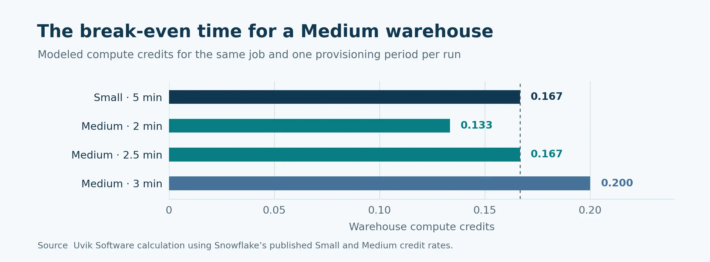
Figure 1. Uvik Software’s warehouse sizing model. A five-minute Small run and a 2.5-minute Medium run both use about 0.167 credits under the stated conditions. Snowflake’s published credit rates
Use this calculation to decide which size to test. Compare complete windows after a resize so you catch queues, concurrent jobs, cache effects, and idle intervals. Calculate the cost using metered credits divided by successful jobs. Include separately billed acceleration where it affects the decision.
Rank query families inside the highest cost warehouse
This example uses the same date window as the warehouse summary. Replace the example warehouse ID with an ID from the first query, then map the top tags to actual owners. Query history data adds queue duration and workload context. Use attributed count as the denominator for this query view, and join job-level outcomes separately for the cost-per-successful-run measure.
SET audit_warehouse_id = 12345;

SELECT h.warehouse_id,
       COALESCE(NULLIF(h.query_tag, ''), 'untagged') AS workload,
       h.query_parameterized_hash AS query_family,
       COUNT(*) AS attributed_queries,
       ROUND(SUM(a.credits_attributed_compute), 3) AS query_credits
FROM snowflake.account_usage.query_attribution_history AS a
JOIN snowflake.account_usage.query_history AS h
  ON h.query_id = a.query_id
WHERE a.start_time >= DATEADD(day, -29, CURRENT_DATE())
  AND a.start_time <  DATEADD(day, -1, CURRENT_DATE())
  AND h.warehouse_id = $audit_warehouse_id
GROUP BY 1, 2, 3
ORDER BY query_credits DESC
LIMIT 25;
Snowflake documents exceptions in query attribution, including some very short queries and warehouses that use a separate metering view. Use the family-level output to prioritize an investigation. Compare tags, run artifacts, and actual execution plans to explain a change. Reconcile the billing period and warehouse totals separately. Snowflake query attribution usage notes
Join dbt success to the warehouse review
Keep a job run record with the scheduled time, warehouse ID, dbt invocation ID where you record it, required outputs, and success state. The dbt run results artifact exposes the invocation ID in its metadata and per-node outcomes for executed nodes. Use your orchestration record for the job-level outcome, especially when a schedule starts multiple invocations. If joins from tags to run IDs are unavailable, compare scope and time windows explicitly and mark model attribution as partial. dbt run results artifact
Run one change over 30 days
| Days | Work | Evidence to keep |
|---|---|---|
| 1 to 5 | Inventory warehouses and agree ownership, deadlines, and cost boundaries. | Scope sheet with job families, baselines, and sign-off owner |
| 6 to 12 | Review settled usage and select the largest avoidable driver. | Hourly compute and idle breakdown, query attribution, and run IDs |
| 13 to 23 | Run one reversible change across matched windows. | Config diff, release times, run counts, credits, p95 latency, and freshness |
| 24 to 30 | Validate the operating result and decide whether to keep, revert, or expand. | Approval, ongoing budget or monitor, and next review date |
Match the test to the workload’s calendar. Track month-end separately when it changes job mix or data volume. If a warehouse serves both dbt and interactive work, compare both cohorts before expanding the change. The owner can then approve it for the workloads the experiment actually tested.
Calculate the change for a dbt warehouse
The sample analytics warehouse runs 4,000 successful jobs in each matched measurement window. The trial consolidates compatible dbt start times. Finance agrees the audit will use warehouse compute credits and the data owner agrees to a p95 job runtime of at most 8.5 minutes and p95 data freshness lag of at most 12 minutes. The figures are illustrative and reflect the same reporting boundary in both windows.
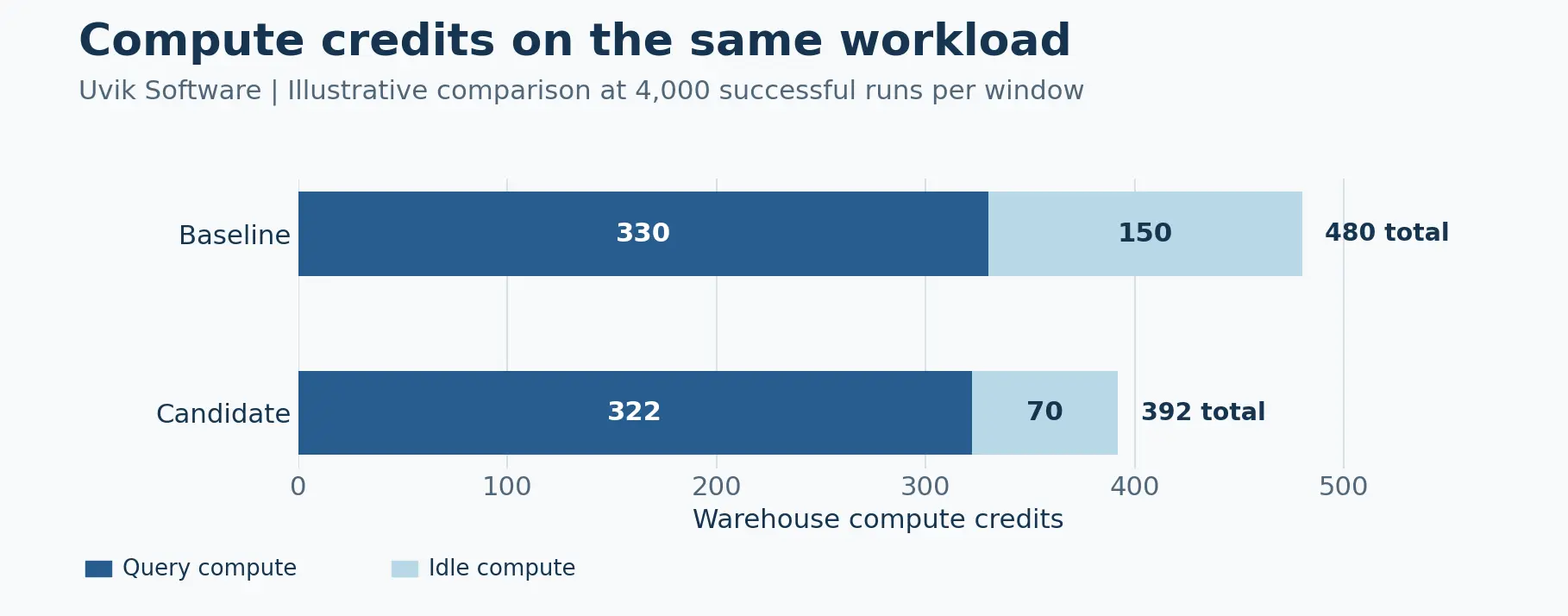
Figure 2. Illustrative Uvik Software compute audit. Warehouse compute falls by 88 credits on matched output volume, with 80 credits of the reduction in idle compute.
| Measure | Baseline | Candidate | Example decision |
|---|---|---|---|
| Warehouse compute credits | 480 | 392 | 88 credits lower, an 18.3% reduction |
| Query compute credits | 330 | 322 | Inspect remaining expensive families |
| Idle compute credits | 150 | 70 | 80 fewer idle credits |
| Successfully completed job runs | 4,000 | 4,000 | Workload denominator matched |
| Compute credits per successful run | 0.120 | 0.098 | 18.3% lower |
| p95 job runtime | 7.8 min | 7.9 min | Passes the 8.5 minute limit |
| p95 data freshness lag | 9.8 min | 10.2 min | Passes the 12 minute limit |
| Missed required finance refreshes | 0 | 0 | Zero permitted for that report in this example |
Idle compute accounts for 80 of the 88 fewer credits, about 91% of the modeled change. That supports keeping the schedule experiment for this warehouse. Compare run counts and retries by job family, then check every required finance deadline. A passing p95 still allows some runs above the threshold.
Make the audit worksheet part of normal ownership
Copy these fields into a row for each warehouse and its critical job families. Give each row one accountable owner and a date for the next review.
| Field | Example entry |
|---|---|
| Warehouse and workload | Analytics ELT and scheduled dbt billing jobs |
| Owner and cadence | Analytics engineering lead reviews weekly and after schedule changes |
| Baseline and candidate windows | Agreed business days with the same dbt job mix |
| Cost measure | Warehouse compute credits per successful run |
| Readiness checks | p95 runtime at or below 8.5 minutes and freshness lag at or below 12 minutes |
| First action and revert | Consolidate compatible runs and restore the old schedules if a required threshold fails |
| Ongoing control | Usage alert with a named Slack or ticket destination and change owner |
Budget alerts and resource monitors serve different operating needs. Use budgets for supported spend visibility. Resource monitors can notify and suspend assigned user-managed warehouses at configured thresholds. Verify the scope against the specific features you use and agree which owners can suspend critical compute. Snowflake documents separate coverage for serverless features and certain warehouse types. Snowflake budgets · Snowflake resource monitors
Read vendor savings figures at their actual scope
Snowflake’s Pfizer case reports 28% lower compute costs after platform consolidation. It separately reports 57% lower total cost of ownership after additional optimizations. For a warehouse tuning test, report the comparison window, successful workloads, credit categories, contractual rate, and missed deadlines. That gives finance a basis for valuing the change and deciding whether to extend it to other warehouses. Snowflake’s Pfizer case study
How Uvik Software assigns responsibilities across the stack
In Uvik Software’s published platform example, Snowflake serves BI and warehouse workloads, dbt owns the transformation layer, and Databricks handles selected heavy compute and ML workloads. That division makes it easier to assign Snowflake warehouse cost and job-level ownership before auditing. The 480-to-392 example above is an illustrative calculation. Uvik Software’s Snowflake, dbt, and Databricks architecture
For help assigning cost and performance to dbt models, see Uvik Software’s analytics engineering services. Bring a warehouse ID, a recent run history export, and the reports that have strict freshness deadlines when you book a Snowflake compute review with Uvik Software.